Chapters · Chapter 6 of 21

Chapter 5 - Text Clustering and Topic Modeling

Clustering documents using a wide variety of language models.

This notebook is for Chapter 5 of the Hands-On Large Language Models book by Jay Alammar and Maarten Grootendorst.

[OPTIONAL] - Installing Packages on

If you are viewing this notebook on Google Colab (or any other cloud vendor), you need to uncomment and run the following codeblock to install the dependencies for this chapter:

💡 NOTE: We will want to use a GPU to run the examples in this notebook. In Google Colab, go to Runtime > Change runtime type > Hardware accelerator > GPU > GPU type > T4.

# %%capture
# !pip install bertopic datasets openai datamapplot

ArXiv Articles: Computation and Language

# Load data from huggingface
from datasets import load_dataset
dataset = load_dataset("maartengr/arxiv_nlp")["train"]

# Extract metadata
abstracts = list(dataset["Abstracts"])
titles = list(dataset["Titles"])

A Common Pipeline for Text Clustering

1. Embedding Documents

from sentence_transformers import SentenceTransformer

# Create an embedding for each abstract
embedding_model = SentenceTransformer('thenlper/gte-small')
embeddings = embedding_model.encode(abstracts, show_progress_bar=True)

# Check the dimensions of the resulting embeddings
embeddings.shape

2. Reducing the Dimensionality of Embeddings

from umap import UMAP

# We reduce the input embeddings from 384 dimenions to 5 dimenions
umap_model = UMAP(
    n_components=5, min_dist=0.0, metric='cosine', random_state=42
)
reduced_embeddings = umap_model.fit_transform(embeddings)

3. Cluster the Reduced Embeddings

from hdbscan import HDBSCAN

# We fit the model and extract the clusters
hdbscan_model = HDBSCAN(
    min_cluster_size=50, metric='euclidean', cluster_selection_method='eom'
).fit(reduced_embeddings)
clusters = hdbscan_model.labels_

# How many clusters did we generate?
len(set(clusters))

Inspecting the Clusters

Manually inspect the first three documents in cluster 0:

import numpy as np

# Print first three documents in cluster 0
cluster = 0
for index in np.where(clusters==cluster)[0][:3]:
    print(abstracts[index][:300] + "... \n")

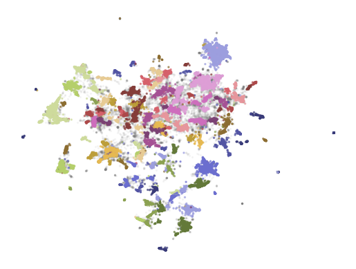
Next, we reduce our embeddings to 2-dimensions so that we can plot them and get a rough understanding of the generated clusters.

import pandas as pd

# Reduce 384-dimensional embeddings to 2 dimensions for easier visualization
reduced_embeddings = UMAP(
    n_components=2, min_dist=0.0, metric='cosine', random_state=42
).fit_transform(embeddings)

# Create dataframe
df = pd.DataFrame(reduced_embeddings, columns=["x", "y"])
df["title"] = titles
df["cluster"] = [str(c) for c in clusters]

# Select outliers and non-outliers (clusters)
clusters_df = df.loc[df.cluster != "-1", :]
outliers_df = df.loc[df.cluster == "-1", :]

Static Plot

import matplotlib.pyplot as plt

# Plot outliers and non-outliers seperately
plt.scatter(outliers_df.x, outliers_df.y, alpha=0.05, s=2, c="grey")
plt.scatter(
    clusters_df.x, clusters_df.y, c=clusters_df.cluster.astype(int),
    alpha=0.6, s=2, cmap='tab20b'
)
plt.axis('off')
# plt.savefig("matplotlib.png", dpi=300)  # Uncomment to save the graph as a .png

From Text Clustering to Topic Modeling

BERTopic: A Modular Topic Modeling Framework

from bertopic import BERTopic

# Train our model with our previously defined models
topic_model = BERTopic(
    embedding_model=embedding_model,
    umap_model=umap_model,
    hdbscan_model=hdbscan_model,
    verbose=True
).fit(abstracts, embeddings)

Now, let's start exploring the topics that we got by running the code above.

topic_model.get_topic_info()

Hundreds of topics were generated using the default model! To get the top 10 keywords per topic as well as their c-TF-IDF weights, we can use the get_topic() function:

topic_model.get_topic(0)

We can use the find_topics() function to search for specific topics based on a search term. Let’s search for a topic about topic modeling:

topic_model.find_topics("topic modeling")

It returns that topic 22 has a relatively high similarity (0.95) with our search term. If we then inspect the topic, we can see that it is indeed a topic about topic modeling:

topic_model.get_topic(22)

That seems like a topic that is, in part, characterized by the classic LDA technique. Let's see if the BERTopic paper was also assigned to topic 22:

topic_model.topics_[titles.index('BERTopic: Neural topic modeling with a class-based TF-IDF procedure')]

It is! We expected it might be because there are non-LDA specific words in the topic describtion such as "clustering" and "topic".

Visualizations

Visualize Documents

# Visualize topics and documents
fig = topic_model.visualize_documents(
    titles,
    reduced_embeddings=reduced_embeddings,
    width=1200,
    hide_annotations=True
)

# Update fonts of legend for easier visualization
fig.update_layout(font=dict(size=16))

# Visualize barchart with ranked keywords
topic_model.visualize_barchart()

# Visualize relationships between topics
topic_model.visualize_heatmap(n_clusters=30)

# Visualize the potential hierarchical structure of topics
topic_model.visualize_hierarchy()

Representation Models

In these examples that follow, we will update our topic representations after having trained our model. This allows for quick iteration. If, however, you want to use a representation model at the start of training, you will need to run it as follows:

from bertopic.representation import KeyBERTInspired
from bertopic import BERTopic

# Create your representation model
representation_model = KeyBERTInspired()

# Use the representation model in BERTopic on top of the default pipeline
topic_model = BERTopic(representation_model=representation_model)

To use the representation models, we are first going to duplicate our topic model such that easily show the differences between a model with and without representation model.

# Save original representations
from copy import deepcopy
original_topics = deepcopy(topic_model.topic_representations_)

def topic_differences(model, original_topics, nr_topics=5):
    """Show the differences in topic representations between two models """
    df = pd.DataFrame(columns=["Topic", "Original", "Updated"])
    for topic in range(nr_topics):

        # Extract top 5 words per topic per model
        og_words = " | ".join(list(zip(*original_topics[topic]))[0][:5])
        new_words = " | ".join(list(zip(*model.get_topic(topic)))[0][:5])
        df.loc[len(df)] = [topic, og_words, new_words]

    return df

KeyBERTInspired

from bertopic.representation import KeyBERTInspired

# Update our topic representations using KeyBERTInspired
representation_model = KeyBERTInspired()
topic_model.update_topics(abstracts, representation_model=representation_model)

# Show topic differences
topic_differences(topic_model, original_topics)

Maximal Marginal Relevance

from bertopic.representation import MaximalMarginalRelevance

# Update our topic representations to MaximalMarginalRelevance
representation_model = MaximalMarginalRelevance(diversity=0.5)
topic_model.update_topics(abstracts, representation_model=representation_model)

# Show topic differences
topic_differences(topic_model, original_topics)

Text Generation

Flan-T5

from transformers import pipeline
from bertopic.representation import TextGeneration

prompt = """I have a topic that contains the following documents:
[DOCUMENTS]

The topic is described by the following keywords: '[KEYWORDS]'.

Based on the documents and keywords, what is this topic about?"""

# Update our topic representations using Flan-T5
generator = pipeline('text2text-generation', model='google/flan-t5-small')
representation_model = TextGeneration(
    generator, prompt=prompt, doc_length=50, tokenizer="whitespace"
)
topic_model.update_topics(abstracts, representation_model=representation_model)

# Show topic differences
topic_differences(topic_model, original_topics)

OpenAI

import openai
from bertopic.representation import OpenAI

prompt = """
I have a topic that contains the following documents:
[DOCUMENTS]

The topic is described by the following keywords: [KEYWORDS]

Based on the information above, extract a short topic label in the following format:
topic: <short topic label>
"""

# Update our topic representations using GPT-3.5
client = openai.OpenAI(api_key="YOUR_KEY_HERE")
representation_model = OpenAI(
    client, model="gpt-3.5-turbo", exponential_backoff=True, chat=True, prompt=prompt
)
topic_model.update_topics(abstracts, representation_model=representation_model)

# Show topic differences
topic_differences(topic_model, original_topics)

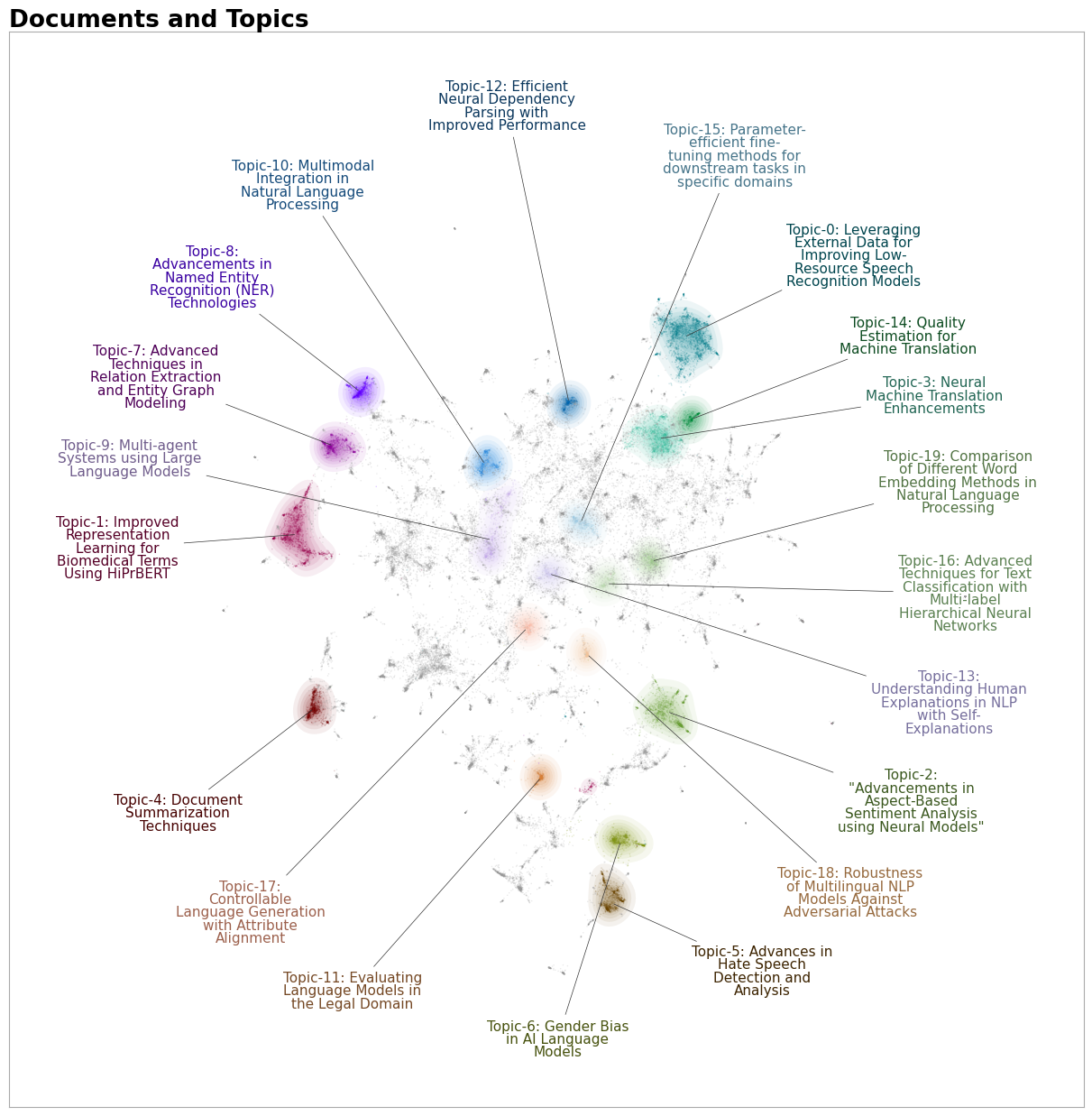
# Visualize topics and documents
fig = topic_model.visualize_document_datamap(
    titles,
    topics=list(range(20)),
    reduced_embeddings=reduced_embeddings,
    width=1200,
    label_font_size=11,
    label_wrap_width=20,
    use_medoids=True,
)
plt.savefig("datamapplot.png", dpi=300)

BONUS: Word Cloud

Make sure to pip install wordcloud first in order to follow this bonus:

First, we need to make sure that each topic is described by a bit more words than just 10 as that would make for a much more interesting wordcloud.

topic_model.update_topics(abstracts, top_n_words=500)

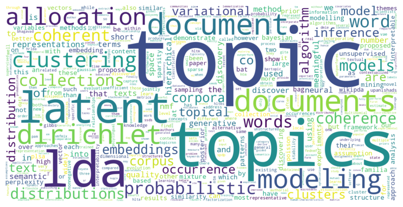
Then, we can run the following code to generate the wordcloud for our topic modeling topic:

from wordcloud import WordCloud
import matplotlib.pyplot as plt

def create_wordcloud(model, topic):
    plt.figure(figsize=(10,5))
    text = {word: value for word, value in model.get_topic(topic)}
    wc = WordCloud(background_color="white", max_words=1000, width=1600, height=800)
    wc.generate_from_frequencies(text)
    plt.imshow(wc, interpolation="bilinear")
    plt.axis("off")
    plt.show()

# Show wordcloud
create_wordcloud(topic_model, topic=17)